I Watched Eric Jang Rebuild AlphaGo So You Don't Have To

In April, Eric Jang spent two weeks rebuilding AlphaGo Zero from scratch, and put the result online as autogo along with a long, interactive write-up. Last week he sat down with Dwarkesh Patel for a two-and-a-half hour blackboard lecture on what he learned. The thread that holds the conversation together is a question about what the AlphaGo recipe still has to teach us in a world where the dominant paradigm has shifted to large language models trained with policy-gradient RL.

This post walks through the ten conceptual blocks of that conversation, in the order they were laid out, with one important correction Eric issued as an errata after recording. The aim is to understand what makes AlphaGo's training loop so elegant, why nobody has been able to port it cleanly to LLMs, and what the limits of current RL look like once you take the AlphaGo perspective seriously.

Contrary to what the title suggests, if you're interested in this type of work, I advise you to watch the podcast episode.

1. Why brute-force search dies on Go

Go is decided by territory under Tromp-Taylor scoring, which is the rule set computer scientists actually use because it has no ambiguity about when a game ends. This matters more than it sounds: it means the AI has a clean reward signal at terminal states, which the human pro game does not have (humans resign).

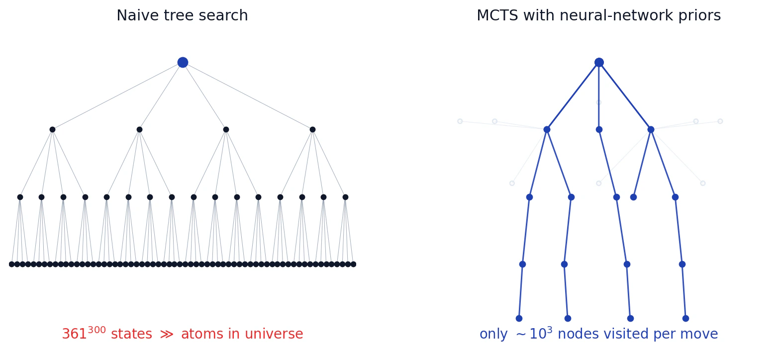
On a 19×19 board there are at most 361 legal moves at the opening, and the branching factor decreases by one each ply because pieces don't move. Games run roughly 300 plies under Tromp-Taylor. The naive game tree therefore has on the order of leaves, which is more states than there are atoms in the observable universe.

Naive Go tree explosion

This is the situation any tabula-rasa Go program walks into. You cannot enumerate. You have to decide which branches are worth exploring. Eric frames the breakthrough of AlphaGo as a tractable answer to two coupled questions: how do you prune the breadth of the tree (which moves to even consider), and how do you prune the depth (when to stop simulating and just estimate the value of the resulting position).

Classical Monte Carlo Tree Search before AlphaGo handled the first question with UCB1 (Upper Confidence Bound 1), a multi-armed-bandit heuristic that selects the child node maximizing

A few definitions I had to nail down to make sense of the data structures:

root node: the current state of the board.
children: the states reachable from the root by one legal move.
: the mean value of leaves reached through this edge.
: the probability of taking action from (this only enters once we have a policy network).

The first term is the exploit term, an online running mean of leaf values reached through that edge. The second is the explore bonus, which grows in proportion to the parent's visit count and shrinks with this child's visit count . UCB1 has regret bounds, and it gives you a principled way to allocate simulations across branches.

The trouble is that UCB1 has no opinion about which children are a priori worth visiting. With 361 candidate moves, you waste an enormous number of simulations early, sampling stupid moves the same way you sample promising ones. Eric's framing here is sharp: classical MCTS treats every action as a uniform prior over a wide bandit. That is fine for a 10-armed bandit. It is hopeless for a 361-armed one with 300 levels of nesting.

2. PUCT, and why the prior is the whole game

AlphaGo's first major change is to swap UCB1 for PUCT (Predictor + Upper Confidence applied to Trees):

PUCT formula

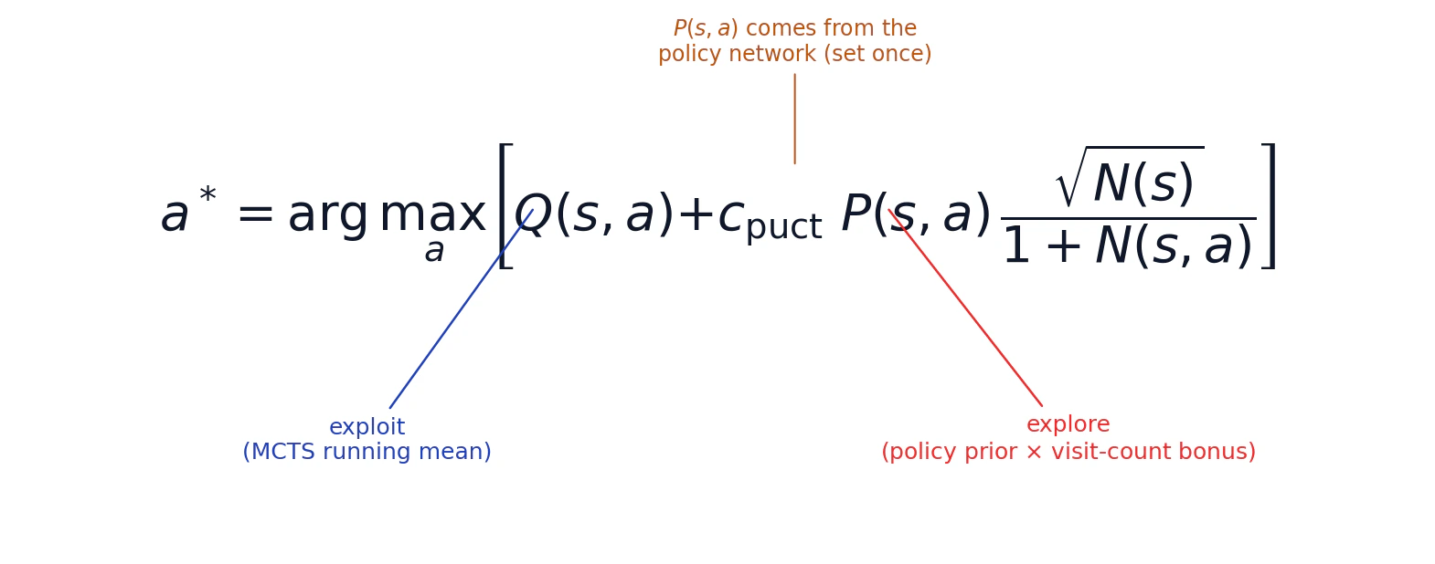
The new term is , the policy prior. This is the probability assigned to action by a neural network evaluated at , and it is written into the tree node exactly once, at the moment that node is expanded. Everything else in the formula remains a search-time statistic: is the running mean of leaf values, is the parent's visit count, is this edge's visit count.

On the first visit to a new node, , so the explore term reduces to . Children with high prior get visited first. As you keep visiting a child, in the denominator grows linearly while in the numerator grows only as a square root, so the explore term decays and takes over. The prior thus determines the order in which children are tried; visit counts determine when you stop trying them; and takes over as soon as the search has enough evidence.

In a Go bot trained from scratch, the prior carries roughly all the search-time information about which moves are not obviously stupid. The value head tells you when to stop searching. Without a good prior, MCTS still spreads itself across all 361 moves and the search depth never becomes tractable. This chapter handles breadth, depth is handled by a second output of the network, the value head.

3. The two-headed network

As Eric puts it: humans look at the board and instinctively calculate the probability of winning 100 moves before the game ends. A neural network can amortize that calculation, replacing a 100-move rollout with a single forward pass. Once you have a value head, you do not have to simulate to the leaf; you just stop at any non-terminal state and trust the value head's prediction.

AlphaGo's neural network takes a board state and outputs two things:

Policy head, : probability distribution over good actions. Prunes breadth.
Value head, : probability of winning from this state. Prunes depth.

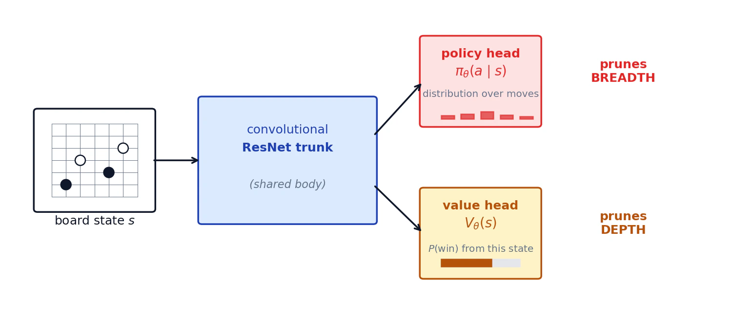
AlphaGo two-headed policy and value network

A natural question is whether the policy head is even necessary. If tells you the probability of winning from any state, why not just enumerate the next states that follow from each legal move , evaluate on each, and play the move with the highest value? Two reasons that come up in the lecture. First, this requires running the network forward up to 361 times per move, where one forward pass of the policy head gives you all the move probabilities at once. Second, an argmax over values is a single point estimate; the whole point of training is to distill what MCTS computed (which is more than a single argmax) back into the policy network. A single forward pass cannot encode a search.

A second, more architectural question that comes up: why convolutional ResNets, when the rest of the field has moved to Transformers? Eric tried Transformers at his scale and could not beat ResNets. His read is that Go fighting (captures, ladders, life-and-death problems) is intensely local. Convolutional receptive fields encode "what is near this stone matters most," and a useful local pattern is reused across the board. At larger scales he expects Transformers can learn this inductive bias from data, but at the budget he was working at, the CNN prior won.

And finally, the network sees only the current board, not the history. Go is a perfect-information game and there is a Nash equilibrium strategy that depends only on . In hidden-information games like poker or Diplomacy, the value of your hand depends on opponents' earlier bluffs or alliances, and you need an architecture that carries state across time. For Go, you do not.

4. Self-play and what gets distilled

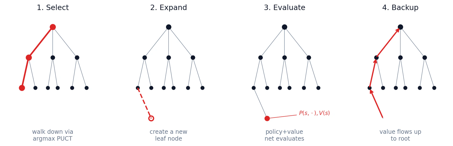
Once you have the network and PUCT, the training loop is simple. For each move in each self-play game, the agent does simulations of MCTS (Eric used numbers from 200 to 2048, the upper range matching KataGo). The four steps of one simulation are: select a path down the tree via argmax PUCT until you reach an unexpanded leaf; expand by adding the leaf as a node; evaluate by running the network on the leaf to get and ; back up by walking the value back to the root, incrementing visit counts and updating 's running mean at each edge.

Four steps of Monte Carlo Tree Search

After all simulations from a given root, the agent picks a move (proportional to root visit counts during training, argmax at inference) and records two things for that state: the MCTS visit distribution , and the final game outcome relative to the side to move. These tuples go into a replay buffer.

Training, then, is just supervised learning on the buffer:

That is it. No advantage estimation, no TD (Temporal Difference) learning, no PPO (Proximal Policy Optimization), no off-policy importance weights. Just a cross-entropy loss against the MCTS visit distribution and an MSE loss against the game result, scaled to taste.

AlphaGo self-play training loop

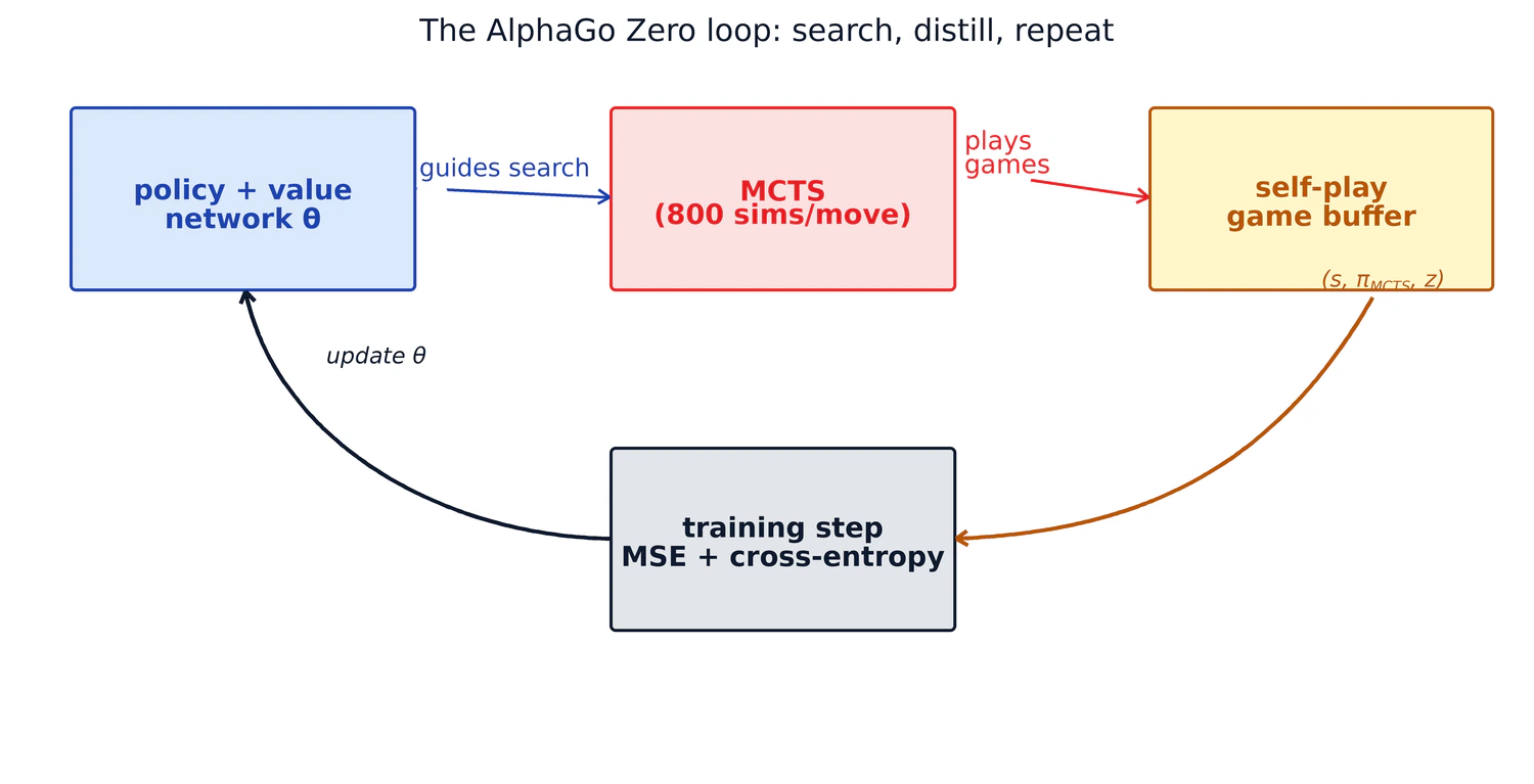
After many rounds, the policy network has internalized what MCTS would have computed at every state it has seen. Forward passes through the network alone get progressively closer to the search distribution, which means the next round of MCTS starts from a sharper prior, which means the search is more efficient, which means the visit distribution is sharper still.

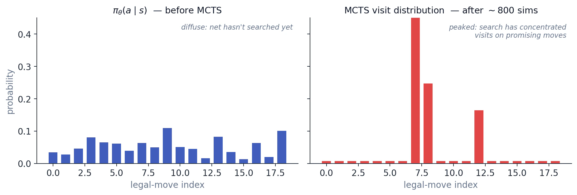
Policy before and after MCTS distillation

You can see why this is so much better than naive winner-imitation. The MCTS-distilled policy benefits from search at every state, not just at terminal positions where you found out you won. The win-rate curves below illustrate the gain: even with a single forward pass and no MCTS at inference, a network trained on MCTS targets is much stronger than one trained on game outcomes alone. With MCTS layered back on at inference, you get another lift on top of that.

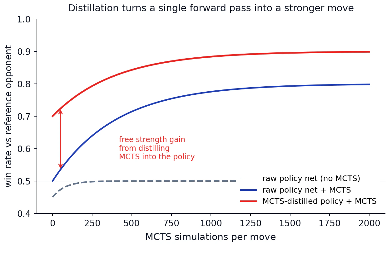
Win rate curves for policy and MCTS agents

The dashed line is a raw policy network with no MCTS at all. The blue line is the same network with MCTS layered on. The red line is a network that has been distilled on MCTS targets, with MCTS again layered on at inference. Even at zero MCTS sims, the distilled network is much stronger. Distillation has packed the search into the forward pass.

Eric calls AlphaGo "elegant" several times during the lecture, and this is what he means. You are always operating in a regime where the supervision signal is clean and dense, because MCTS is giving you a strictly better label at every state you visit, not just at the few states that happened to lead to a win. As he puts it near the end of the podcast: in AlphaGo, you never have to solve the exploration problem of "how do I get to a non-zero success rate." Every step is a hill-climb on a beautiful supervised signal.

5. Why naive REINFORCE plateaus

To see why AlphaGo/MCTS distillation is special, the lecture detours through what doesn't work. Suppose you skipped MCTS entirely and just did naive policy-gradient self-play: play a league of policy checkpoints against each other, find the games where one side won, and reinforce the actions in those games.

Eric's worked example: two evenly matched policies play 100 games of 300 moves each. By luck, one of them wins 51 to 49. Imagine only one of those 51 wins came from a genuinely better move; the other 50 are statistical noise. The naive REINFORCE update wants to upweight every action in every winning game. So you get one useful gradient buried inside ~30,000 noisy labels.

The variance math:

where . The covariance terms give you worst-case variance in sequence length. This is the "quadratic in " point that comes up later in the LLM discussion.

A correction worth flagging. In the podcast Eric attributes the quadratic blowup to the multi-step formulation of the policy gradient and suggests this is why LLM labs prefer single-step RL. After recording he issued an errata: the variance grows quadratically with sequence length regardless of whether you formulate the gradient over the full sequence or per-token. In fact, with per-token rewards, multi-step RL has lower variance than single-step. The real reason LLM labs do single-step is that they only have sequence-level rewards (did the code pass, did the answer help), so the per-token formulation gives you the same thing. The takeaway is that credit assignment in long sequences is quadratically hard in the worst case, not that the choice of formulation is what causes the blowup.

What MCTS does differently is sidestep the credit-assignment problem entirely. Instead of "this game was won, copy these moves," MCTS says "at every state you visited, here is a strictly better move than the one you played." Every visited state becomes a dense supervision target. There is no noise to dig the signal out of.

The classical fixes for RL variance (advantage estimation , TD learning, Generalized Advantage Estimation) all try to reduce variance by subtracting an estimate of the average performance from the return. They are correct as far as they go. But they are reducing the variance of an already-noisy signal. MCTS replaces the signal entirely with a denser one.

6. MCTS, NFSP, and search in two directions

MCTS is not the only way to assign every visited state a better action. Another option is Neural Fictitious Self-Play (NFSP), used to great effect in DeepMind's AlphaStar and OpenAI Five.

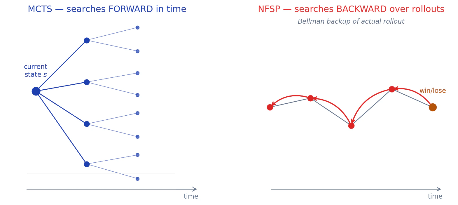
MCTS versus NFSP search directions

In NFSP, you fix an opponent and train a "best response" policy against it using model-free RL (PPO, V-MPO, Q-learning, take your pick). The reward signal is 1 if wins, 0 otherwise. You repeat across different opponents, and you use each best response as a label provider for the corresponding states.

Both MCTS and NFSP produce the same thing: for every state in the replay buffer, an improved action for the student policy to imitate. The difference is where the improved action comes from. MCTS rolls forward in simulated futures and uses the value function to score imagined leaves. NFSP runs actual rollouts to terminal reward, then propagates the win/lose signal backward through TD-style updates over states the agent has actually visited.

MCTS searches forward over imagined trajectories; NFSP searches backward over realized trajectories

The recipe is "label every state in your buffer with a search-improved action and supervise on that." MCTS is the cheapest way to do that in Go because the game is fully observable and you can simulate forward. In imperfect-information games, NFSP achieves the same thing backward.

7. Why MCTS does not transfer to LLMs

The DeepSeek-R1 paper reported that they could not get MCTS to work for LLM reasoning. Eric's diagnosis identifies two structural failures:

Unbounded breadth. Go has at most 361 legal moves per ply. The space of "possible next thoughts in a reasoning trace" is essentially unbounded. PUCT's structure assumes you will visit the same child multiple times to refine its . With language, you almost never sample the exact same continuation twice. The visit-count machinery breaks down.

Depth is unbounded and the value head is hard-to-train. In Go, is the probability of winning a fully specified game from a fully specified position. In LLM reasoning, what is the value of a half-finished proof? Of a partially written function? You cannot easily train a value head on partial reasoning trajectories because there is no clean termination condition and no clean reward.

You could compensate for either one of these. Compensating for both at once is much harder. (People have, with various Tree-of-Thoughts variants). PUCT is a heuristic tuned for the size and depth of Go. It does not gracefully scale to the combinatorics of language.

What does work in current LLMs is something that looks like reasoning without an explicit tree structure: models try one approach, notice it isn't working, back up, try another. This emerged from training rather than being explicitly built. Eric does not rule out a comeback for forward search in LLM reasoning, just probably not as PUCT over tokens. (MuZero-style methods on continuous control are still being pushed.)

A relevant footnote from the conversation: in 2021, Andy Jones published Scaling Scaling Laws with Board Games, which showed you can trade off training compute against test-time compute in MCTS-driven board games at predictable rates. This is the test-time scaling paradigm later popularized by o1-class reasoning models, anticipated five years early on a Go bot. The catch is that scaling laws only emerge once the underlying recipe is working; if your data is bad or your architecture is wrong, scaling laws will give you confidently extrapolated nonsense. Eric started autogo partly to see if you could Bitter-Lesson your way to a strong Go bot using only scaling laws. His honest answer: you cannot, because you need a working system first to generate the data scaling laws fit to.

8. Off-policy training and DAgger

One of the more surprising things about AlphaGo Zero in practice is that its replay buffer is effectively off-policy and it works anyway. By the time you do a gradient step, most (state, action) pairs in the batch were generated by older versions of the policy. RL researchers normally worry about this; off-policy is a known source of instability.

Working through the definitions in my notebook:

Off-policy means the agent learns an optimal strategy by evaluating and improving a policy different from the one that generated the actions. It learns from what other policies (or past selves) did. Q-learning, deep deterministic policy gradient, and soft actor-critic are classic off-policy methods. They are sample-efficient and exploratory but can be unstable.
On-policy means the agent only learns from the actions its current policy produces. PPO is the canonical example.

The puzzle with AlphaGo Zero is: why is the off-policy replay buffer stable?

The answer is DAgger (Dataset Aggregation, from Stéphane Ross's imitation learning work). The failure mode of on-policy imitation learning is that you train only on the optimal trajectory's states; the first time you drift off, you are in a state your training data does not cover, and errors compound. DAgger augments the training set with off-optimal states labeled with the expert action that would funnel you back.

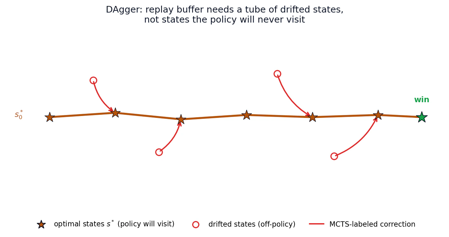
DAgger dataset aggregation diagram

AlphaGo's replay buffer is naturally a DAgger dataset. The states in the buffer are mostly along the policy's typical trajectories, with some drift. Every state in the buffer carries an MCTS-derived label that, by construction, points toward winning. So even when you sample old states, the supervision teaches the network to funnel toward the manifold of winning trajectories.

The failure mode that would break it is if the buffer contained states the current policy would never visit. Then you train on regions of state space irrelevant to actual play. AlphaGo-Zero-style systems keep this in check by mixing in fresh self-play data.

Eric pushed this further in autogo: he ran an experiment where, instead of MCTS-ing every move of a self-play game, he randomly sampled board states and re-ran MCTS on each with the current network. This is much more like a robotics off-policy setup, where a Bellman updater continuously rethinks "what should I have done from this state?" It works. The MCTS labels still funnel back to winning play even from random board states.

This is also the strongest connection between AlphaGo and modern robotics off-policy learning. QT-Opt and similar systems do exactly this: a pusher writes transitions into a replay buffer, a Bellman updater continuously recomputes targets, and a trainer does supervised regression against those targets. AlphaGo just uses search instead of Bellman backups to produce its targets.

9. RL is more information-inefficient than you think

The most quotable section of the podcast comes when Dwarkesh and Eric discuss bits per sample. The standard worry about RL is sample inefficiency: you have to roll out a whole trajectory to get any signal. As agents take on multi-day tasks, samples per FLOP keeps falling.

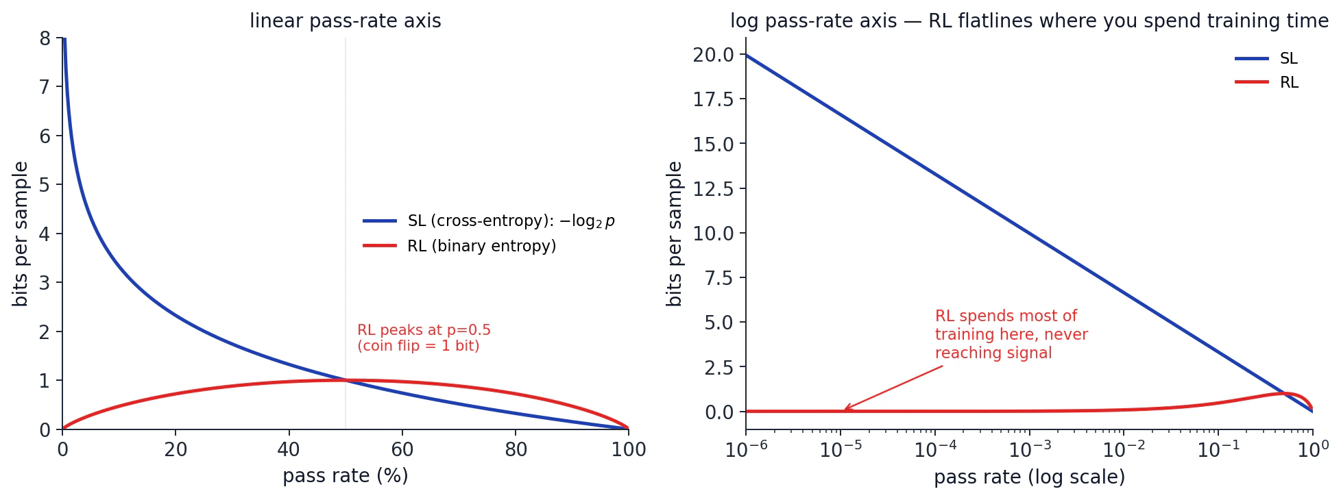
The less-appreciated problem is bits per sample. Imagine an untrained LLM facing the prompt "the sky is..." with vocabulary size 100K. Under supervised learning, you are told the answer is "blue" and your cross-entropy loss is , a large number when your model puts low probability on "blue." Under RL, you have to sample "blue" before you get any signal. With random initialization, your probability of sampling it is roughly . You will need on the order of 100K samples to stumble onto "blue" once. Until you do, every sample teaches you nothing.

Bits per sample comparison

Formally: at pass rate , supervised learning provides bits per sample (huge when is tiny). RL on a binary outcome provides the binary entropy

which peaks at (a coin flip is one bit) and goes to zero at both extremes. You spend almost all of training in the small- regime, where RL gives you nearly zero bits per sample while SL would give you a lot.

This is the deepest reason AlphaGo's loop is special. Every supervision step is a soft target on the visit distribution, not a one-hot on a single best move. Soft targets carry far more information per sample than one-hot labels: this is the dark-knowledge distillation argument. So AlphaGo's policy network gets the maximum bits per sample at every step. And because MCTS is a strictly better labeler than the current policy, the supervision signal is never flat.

A line from the podcast to remember: in AlphaGo, you don't train the policy network to imitate the MCTS action, you train it to imitate the MCTS distribution. The action is one-hot; the distribution is dense. This is dark knowledge.

For this to work, three things have to be true simultaneously: the value function has to be cheap and concrete, the action space has to be small enough for PUCT to behave, and you need a fast simulator. Go has all three. Coding, multi-step reasoning, and most economically valuable tasks have zero of three.

10. What this means for automated AI research

The closing chapter of the podcast pivots from algorithms to research workflow. Eric used coding agents extensively for autogo. His honest report is that current frontier models are good at hill-climbing once a track is defined. They can run a hyperparameter sweep, identify that gradients are small in some layer, suggest a code change, run an experiment, and propose follow-ups. He calls this "grad-student-like" execution on a fixed objective.

What they cannot yet do, and what Eric repeatedly bumps into, is lateral thinking. When the current track is wrong (the metric is plateauing, the infra has a subtle bug, the framing of the problem is off), the models will keep grinding the wrong axis instead of stepping back to first principles. The actual research insight tends to come from the human noticing "wait, this whole branch of experiments is downstream of a misassumption."

This is the inverse of the AlphaGo lesson. AlphaGo works because MCTS gives the policy network a teacher that is always better, on every state. Current LLM coding agents have no such teacher. They have a reward (did the test pass) and a long horizon over noisy intermediate choices. They are in the high-variance, low-bits-per-sample regime that Eric just spent two hours explaining.

If you want a single takeaway from the rebuild-AlphaGo exercise, it is this: figuring out how to give an agent a per-state teacher (some equivalent of MCTS's "here is a strictly better action than the one you played") is probably more leverage than scaling RL on sparse terminal rewards. Whether that teacher comes from forward search, backward TD, distillation from a stronger model, or something we have not invented yet is the open question. But the AlphaGo recipe makes it very clear what we are missing.

Thank you to Eric Jang and Dwarkesh Patel.

Eric's interactive AlphaGo tutorial is the canonical reference, with full code at autogo on GitHub. His errata on policy-gradient variance is short and worth reading.